Logarithms
This Frequently Asked Question (FAQ) tutorial on logarithms is designed to give intro computer science students a refresher on logarithms: what they are, when and why they might be useful, and how to graph them using the Python matplotlib library.
Definition
The logarithm is the inverse of the exponential operation.
If bx = n, then x = logb n.
The logarithm answers the question “to what number would I raise the base to get this value?”
Examples, base-10
A common base for working with algorithms is base-10:
- Because 102 = 100, we can say that log10 of 100 = 2.
- Because 103 = 1000, log10 1000 = 3.
- Because 100 = 1, log10 1 = 0.
- Because 101.4313 = 27, we can say that log10 27 = 1.4313.
Additional examples, working the other way:
- log10 100,000 = 5, because 105 = 100000.
- log10 1 = 0, because 100 = 1.
- log10 50 = somewhere between 1 (because 101 = 10) and 2 (because 102 = 100).
log10 50 comes out to be around 1.7, because 101.7 = 50.
Logarithms in base-2
When working with computers, it’s common to use base-2 instead of base 10, particularly when analyzing algorithms. This is because problem-solving strategies that use a divide-and-conquer process can be easily described using base-2 values.
A list of n sorted values, for example, can be divided in half log2 n times to get to a single value.
Example: n = 9 items in a list, divided in half 3 times:
Original list: 2, 5, 8, 9, 13, 15, 21, 26, 29
Division one: 2, 5, 8, 9, 13
Division two: 2, 5
Division three: 2
Example, base-2
- Because 25 = 32, log2 32 = 5.
- Because 20 = 1, log2 1 = 0.
- Because 23.7 = 13, log2 13 = 3.7.
Or, working the other way:
- log2 16 = 4, because 24 = 16
- log2 256 = 8, because 28 = 256
- log2 1000 = 9.967, because 29.967 = 1000
Where is the log2 button on my calculator?
There probably isn’t one, but you can calculate it using the standard log button, which is log10. Because
logb a = logd a / logd b
we can see that
log2 a = log10 a / log10 2
So, to calculate log2 28, you would enter
log10 28 / log10 2
Why logarithms are useful
Some progressions of numbers can be easily understood in a summative way: adding n more items to a pile of existing items increases the total number of items in the pile by an amount n.
Other series can be better understood in a multiplicative way: increasing the pile by a factor of 10 (n1) yields a smaller pile than if we increased the pile by a factor of 100 (n2).
For situations where a range of values covers a larger scale, using logarithms can help us better understand the way in which those values are changing.
Example
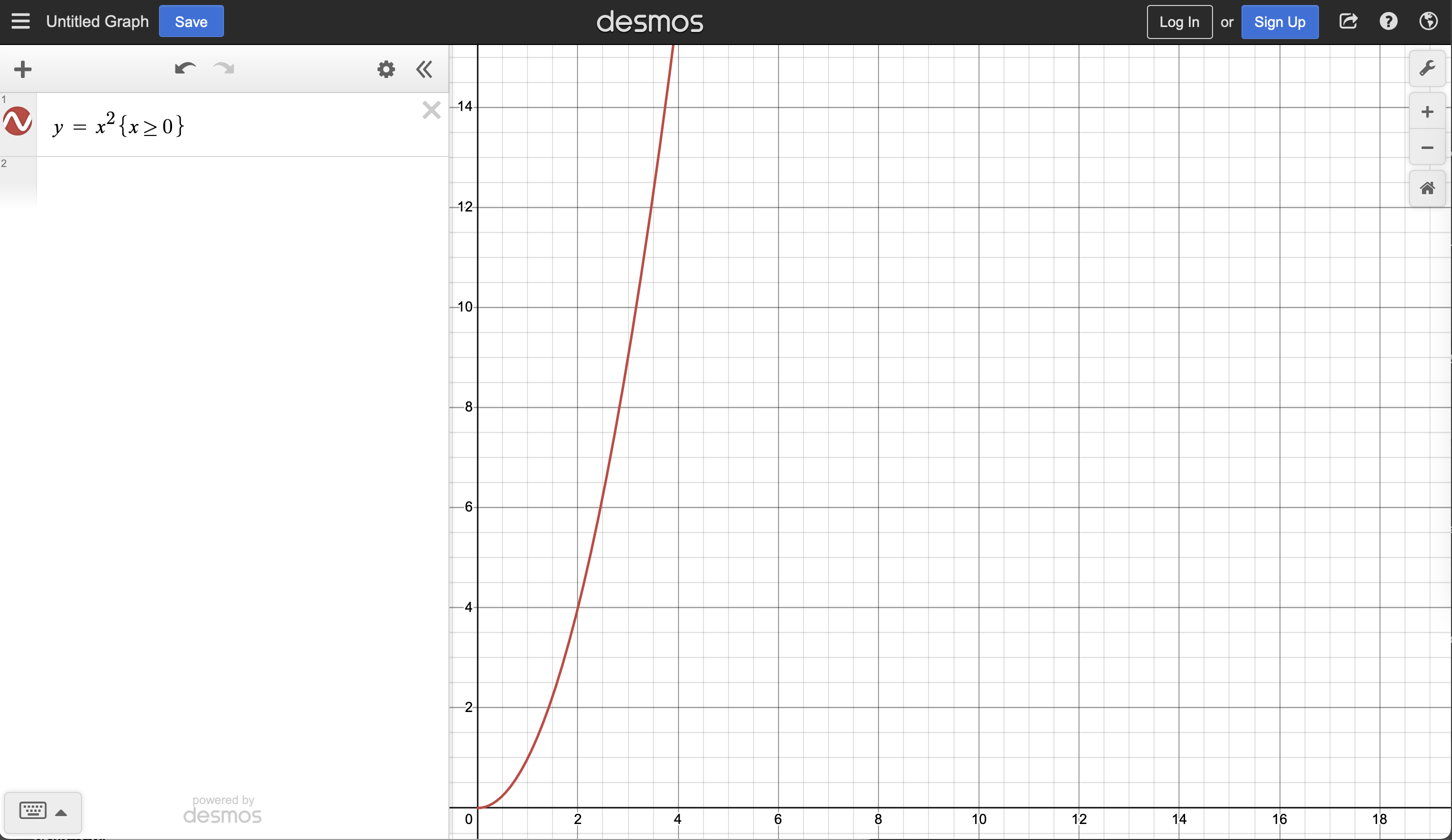
Examine this graph of y = x2 (below). We can see the behavior of the function pretty well on the graph, but the y-axis shoots up so quickly, we aren’t able to use as much of the x-axis to to interpret the graph. The scales on the axes are linear scales where each tick mark along the axis indicates an equal increment.
Now examine this graph of the same function, y = x2, but plotted on a “log-log” scale (ie. a logarithmic scale for both x and y-axes). Each tick mark along these axes represents not a linear increase but a factor increase: the tick distance between the values 1 and 10 is the same as the tick distance between 10 and 100, and 100 and 1000, and 1,000 and 10,000.
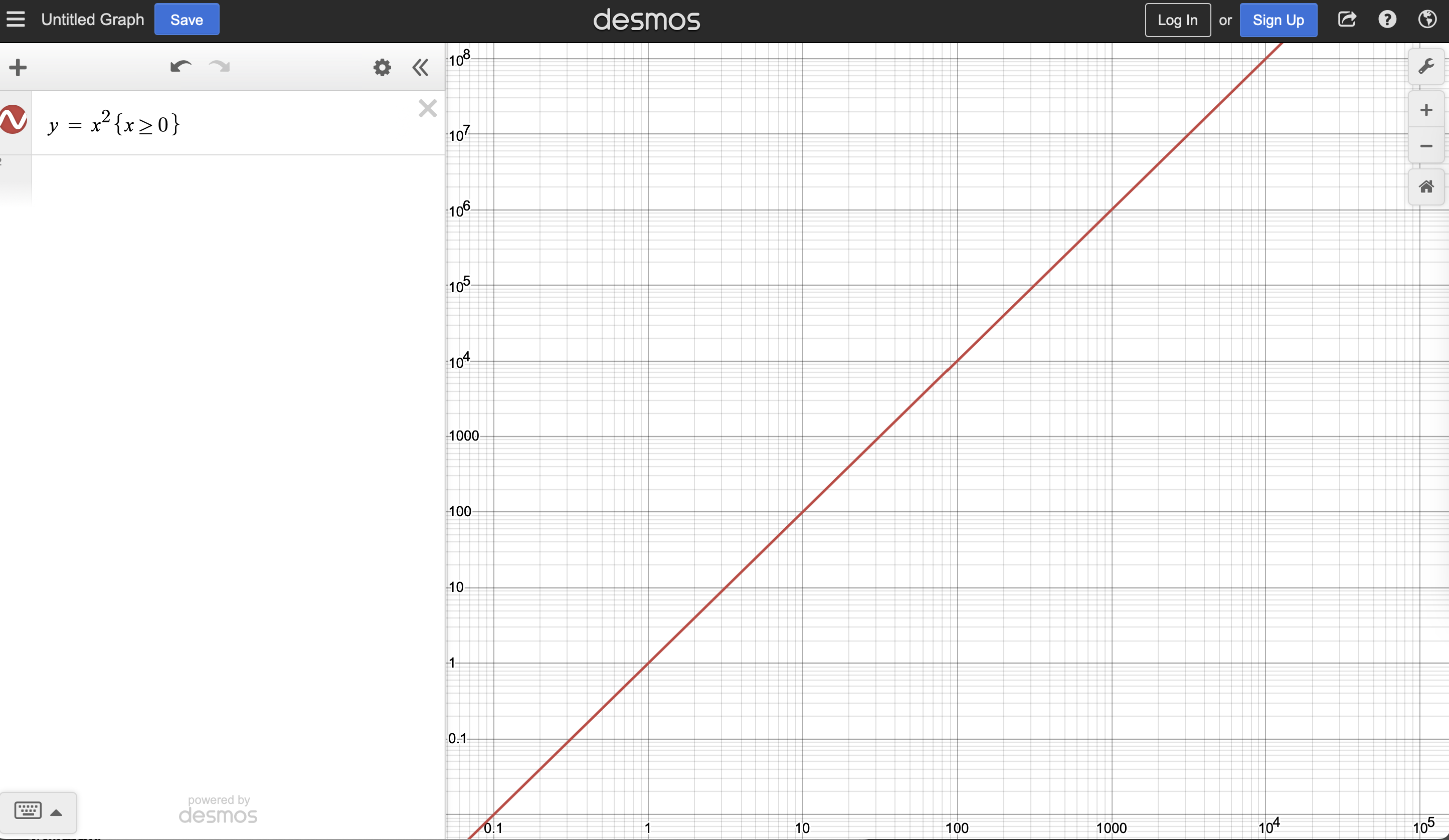
A lot of systems in nature behave as power functions or exponential functions, and it’s common to see graphs of these behaviors with logarithmic scales on one or both axes.
Axis scales for the computer scientist
As mentioned early, many algorithms have a performance related to the log of some value—log n, perhaps, or sometimes n log n (n times the log of n). If we have performance data (execution times for a series of increasingly large data sets, for example) and we want to identify it as behaving according to n log n, plotting that data on a log-log graph does not yield a straight line. A straight line on a log-log graph would reveal a power relationship, not a log relationship.
If we expect n log n behavior, however, we can plot performance time versus n log n. If time goes up linearly, it provides evidence that the performance time varies linearly as a function of n log n.
Example
A complete function showing how to create a sort time vs. n log n plot is given here, along with the corresponding output after running it with an implementation of the Quicksort algorithm.
def produce_graph(test_sizes, times):
    """This function takes a list of test_sizes and
    a corresponding list of times to complete sorting
    the elements of the given size, and produces a
    "time vs. n log n" plot to attempt to identify if
    there is a linear relationship, ie. the algorithm
    has a behavior of O(n log n).

    Requires the scipy stats package, numpy, matplotlib, math, and
    os libraries to be imported. Example import:

        import time
        import random
        import math
        import os
        import matplotlib.pyplot as plt
        import numpy as np
        from scipy import stats
    """

    # create numpy array of calculated `n log n` values
    n_log_n = np.array([test *  math.log(test, 2) for test in test_sizes])

    # create numpy array of the times to sort
    times = np.array(times)

    # set up figure that we can save later
    fig = plt.figure()
    plt.title('Time vs n log n for Quicksort')
    plt.ylabel('sort time (seconds)')
    plt.xlabel('n log n, for array size n')

    # put data on figure, 'bo' = blue dots
    plt.plot(n_log_n, times, 'bo')

    # use scipy to do linear regression on data
    slope, intercept, rval, pval, stderr = stats.linregress(n_log_n, times)

    # plot the regression line
    plt.plot(n_log_n, slope * n_log_n + intercept, color='red')

    # put the regression formula and the R^2 value on the graph
    plt.annotate("y=%.5Ex+%.5E\nR$^2$=%.5f"%(slope, intercept, rval**2), xy=(0.15,0.75), xycoords='figure fraction')

    # Save the plot in a directory called plots
    if not os.path.exists('plots'):
        os.mkdir('plots')
    fig.savefig('plots/quicksort_performance.png')

    # Show the graph on screen
    plt.show()
The resulting graph:
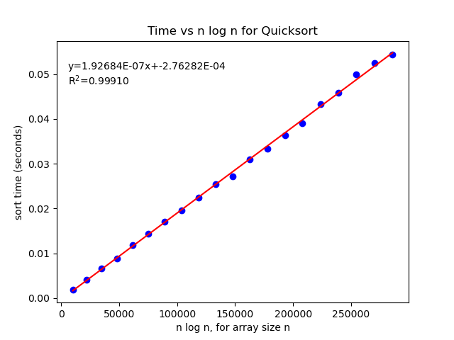
Given the high R2 value, which suggests a strong correlation between the data that was collected and the linear regression model given, we have good evidence that Quicksort, on average, has a performance of O(n log n).